


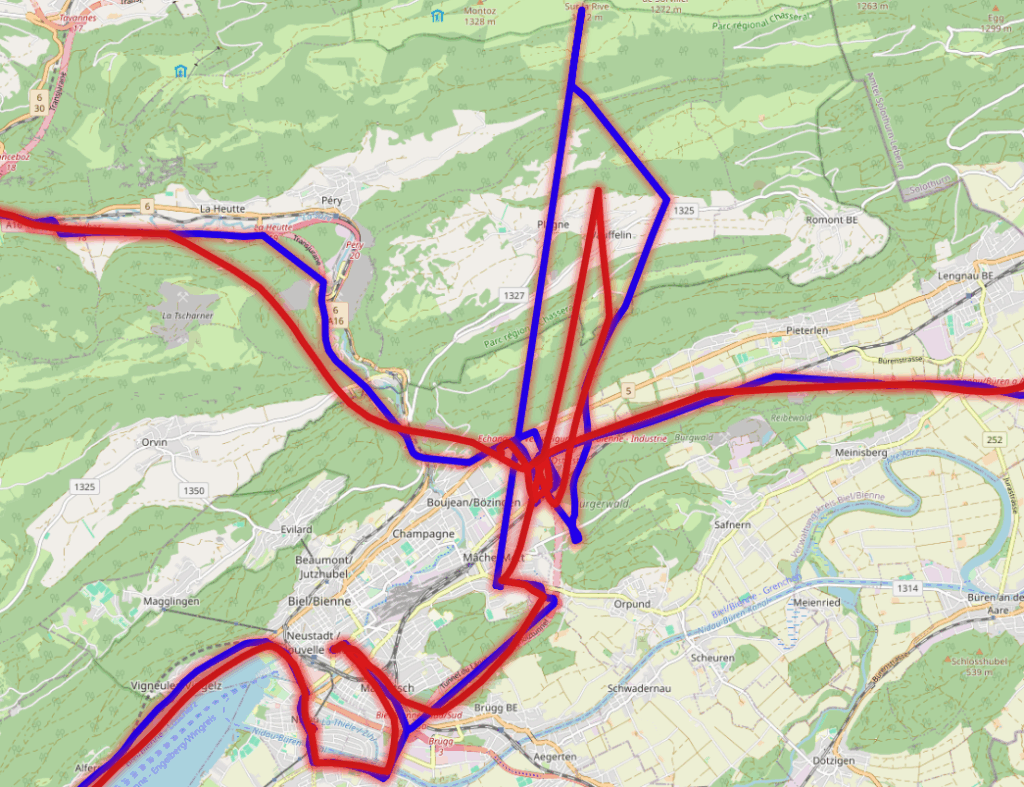
Modern GPS datasets are notoriously noisy: satellites drift, buildings scatter signals, and consumer devices introduce frequent errors. When working with millions of position samples from vehicles, smartphones, or IoT devices, this noise makes analysis unreliable. Routes jump, tracks zigzag, and outliers distort aggregates.
The Kalman Filter is the standard technique for smoothing such data. Traditionally, it is applied outside the database in environments like Python or MATLAB. But for large-scale datasets stored in Postgres, filtering directly inside the database has clear advantages: no additional processing pipeline, results available immediately in SQL, and scalable analytics over billions of rows.
For our own usage at traconiq, we built an open source project that implements a Kalman Filter in Postgres. You can explore the code and try it yourself here, if you also have GPS data:
github.com/traconiq/kalman-filter-neon
Background: What’s a Kalman Filter?
The Kalman Filter is a recursive algorithm used to estimate the true state of a dynamic system, such as the position of a moving vehicle, from noisy observations. At each step, it combines two parts:
- Prediction: uses a motion model to project the next position (and optionally velocity).
- Update: corrects that prediction using the latest observed measurement.
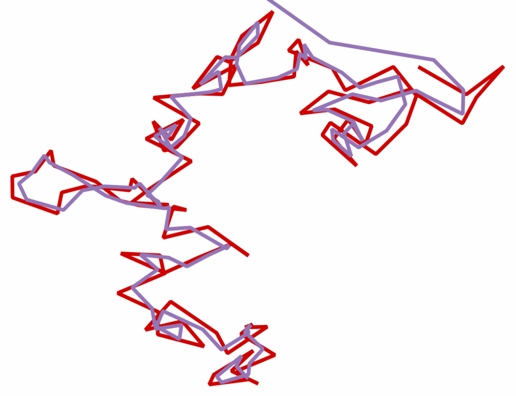
What makes the Kalman Filter effective is that it explicitly models uncertainty. Both the process (how the system evolves) and the measurements (GPS fixes) carry noise, represented in a covariance matrix. The filter continually refines its estimates as new data arrives, producing a smoothed track that follows the real trajectory more closely than raw GPS data.
Because of this, Kalman Filters are widely used in navigation, robotics, signal processing, and finance. Applied to GPS data, they can turn jittery position samples into realistic paths suitable for analytics or visualization.
The Project: Implementing a Kalman Filter in Postgres
The challenge of doing this in SQL
Implementing a Kalman Filter inside Postgres comes with a few difficulties. Unlike procedural languages, SQL does not naturally keep track of “state” across rows, and the filter depends on carrying forward information from one step to the next.
Three requirements in particular need to be addressed:
- State: the filter must store not only the last position estimate but also the covariance matrix that describes its uncertainty. Both are required to compute the next estimate.
- Transition: for each new measurement, a user-defined function must update the state. This function can incorporate additional sensor data when available, such as the reported accuracy (HDOP) or measured speed, to adjust or even skip an update.
- Sequencing: GPS points must be processed in strict time order. The filter only works if each step builds on the previous one, which means queries need to respect record order.
For online filtering, state can be stored per device and updated with each insert. For offline filtering across historical tracks, the sequential nature of the filter makes it harder to implement efficiently in SQL, and requires more advanced techniques.
How we did it
All code in this repo: github.com/traconiq/kalman-filter-neon
Schema
The script example-schema.sql sets up a schema called kalman with two core tables. This design ensures that the state (estimate + covariance) needed for the next filter step is always available:
kalman.positions: stores raw GPS points as well as the filtered positions created during online filtering.kalman.devices: stores device information, including the last known position estimate and covariance matrix for each device.
Functions
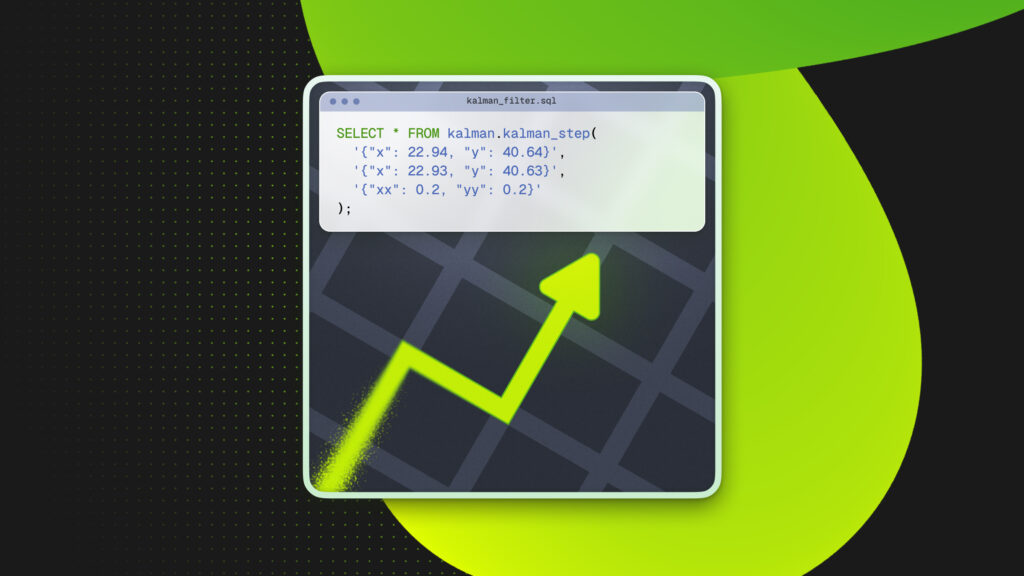
The main function to perform the Kalman step is kalman.kalman_step: it takes the previous estimate and covariance, along with the current measurement, and returns an updated estimate. For online filtering, a wrapper function (kalman.kalman_upsert_position) handles inserts a new GPS point into kalman.positions and simultaneously applies the Kalman step, updating the device’s state in kalman.devices.
Online filtering vs offline filtering
Online filtering is applied as each GPS point is inserted. This ensures smoothed positions are always available, but it comes at the cost of higher insert latency.
Offline filtering is applied later, in batch, across a history of positions. This can be done in two ways:
- Recursive CTEs: step through ordered GPS history, carrying the filter state forward record by record. Transparent, but slower.
- Custom aggregates: repeatedly apply the filter under the hood as rows are combined. More efficient for large-scale postprocessing and fits naturally into SQL analytics.
Benchmarks
TL;DR
Online filtering is practical if you need filtered positions available immediately, but more expensive per insert.
Offline filtering is best done with custom aggregates for efficiency. Recursive CTEs are useful for debugging and transparency but not optimal for production-scale workloads.
Of course, we wanted to measure performance. We run four pgbench scripts:
benchmark_insert_nofilter.sqlto insert GPS points without filteringbenchmark_insert_upsert.sqlto insert GPS points with online filteringbenchmark_offline_recursive.sqlfor offline filtering via a recursive query.benchmark_offline_aggregate.sqlfor offline filtering via a custom aggregate
All benchmarks were run on the same machine and dataset, using pgbench -f <script>.sql -t 1000.
The results show that applying the filter during inserts is feasible but comes with a significant performance penalty: throughput drops by about 35 – 40%. For applications where smoothed data must be immediately available, this tradeoff may be acceptable.
| Test | INSERT NO FILTER | INSERT WITH FILTER |
|---|---|---|
| number of clients | 1 | 1 |
| number of transactions | 1000 | 1000 |
| latency avg (ms) | 8.543 | 13.560 |
| tps (excluding connections) | 117.048322 | 73.743893 |
Benchmark: Online filtering during insert
When comparing it to the offline filtering method, the difference is clear. Recursive queries work, but they add considerable overhead. Custom aggregates, by contrast, achieve higher throughput and are therefore the preferred method for large datasets or batch processing.
| Test | Offline recursive | Offline aggregate |
|---|---|---|
| number of clients | 1 | 1 |
| number of transactions | 1000 | 1000 |
| latency avg (ms) | 0.290 | 0.226 |
| tps (excluding connections) | 3442.637060 | 4419.401171 |
Benchmark: Offline filtering via recursive query vs aggregate
Example usage
This script provides a complete demonstration of how the Kalman Filter can be used directly inside Postgres for both real-time smoothing and large-scale postprocessing.
Try It yourself
You can explore the full implementation in the repo: github.com/traconiq/kalman-filter-neon
To get the feel for it,
- Run
example-schema.sqlto create the schema, tables, and functions - Load
example-usage.sqlto insert sample data and see online and offline filtering in action. - Experiment with the benchmark scripts (
benchmark_insert_nofilter.sql,benchmark_insert_upsert.sql,benchmark_offline_recursive.sql,benchmark_offline_aggregate.sql) to compare performance in your own environment.
Run it on Neon
Neon’s serverless architecture is great to test recursive queries and aggregates on large datasets, while autoscaling and branching let you experiment without extra setup. Spin up a free Postgres database instantly for free and point your client to the Neon connection string to get started.